Monte Carlo Thinking: Simulate Your Portfolio, Don't Predict It

Monte Carlo simulation is a method for answering questions by running them thousands of times with randomness included, then looking at the full range of outcomes instead of a single estimate. It shows up everywhere from engineering to election forecasting, but I find it most useful in personal finance, where the standard way of projecting a portfolio quietly hides most of the risk.

The topic has been on my mind because of a recent project. I built a Monte Carlo engine from the ground up to model churn, growth, and other business motions, drawing on historical distributions, and it now feeds into financial forecasts we make at my day job. Watching it work convinced me the method deserves a bigger place in personal finance too.

I'm also at the very beginning of building a smaller simulator of my own for exactly that (a side project I expect to poke at for months). Writing this post is partly my way of making sure I understand the foundations before I write any code.

The Problem With Averages

If you have ever tried to answer "what will my portfolio be worth in ten years?", you probably reached for an average. Stocks return about 10% a year historically, so you compound that out and get a clean number. For $10,000 invested over ten years, that math says roughly $26,000.

The problem is that nobody experiences the average. Each investor lives through exactly one sequence of returns, and those sequences vary wildly. The average is a summary of thousands of possible futures, most of which look nothing like the summary.

What Is Monte Carlo Simulation?

The method has a fun origin: Stanislaw Ulam dreamed it up in 1946 while recovering from an illness and playing solitaire, when he realized he could estimate his odds of winning by simply dealing out hundreds of hands and counting. Applied to a portfolio, the recipe looks like this:

• Model the inputs: historical returns, their volatility, and how they move together.
• Simulate one future: draw a random sequence of yearly returns from that model.
• Repeat: run the same portfolio through 10,000 of these alternate histories.
• Read the distribution: look at the median, the tails, and everything in between.

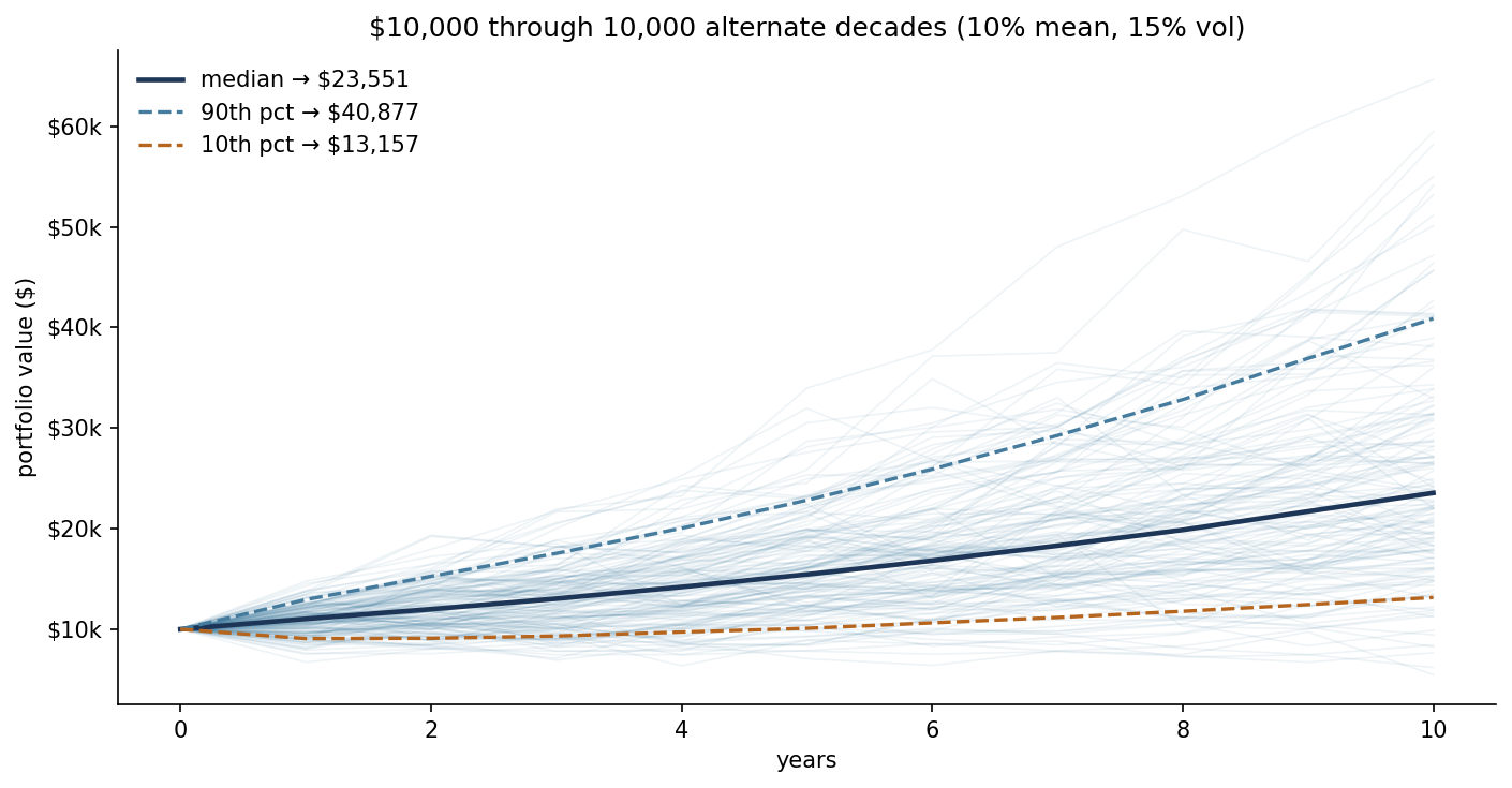
Example: Take that same $10,000 in an index fund, modeled at a 10% average return with 15% volatility. Across 10,000 simulated decades, the average outcome does land near the $26,000 the simple math promised. The typical outcome comes in lower: the median path ends around $23,600, because volatility drags the middle of the distribution below the average. And the spread is wide. In the bottom 10% of simulations you end up near $13,000, and in the top 10% above $41,000. Same investment, same assumptions.

Why It Matters

The spread between those paths is not statistical noise. It contains the two things that actually determine whether an investor sticks with their plan:

• Sequence risk: Two paths can have identical average returns and feel completely different depending on when the bad years arrive. A crash in year one of retirement withdrawals does far more damage than the same crash in year nine, because you are selling shares at the bottom to fund the withdrawals.
• Ruin probability: An average return of 10% is little comfort on the paths where a deep drawdown forces you to sell, whether for emotional or cash-flow reasons. A simulation counts how often that happens instead of assuming it away.

There is a psychological angle here too. We habituate to numbers we hear repeatedly: after enough repetitions, 10% a year starts to feel like a promise rather than a summary statistic. Watching a thousand simulated paths spread apart is a useful corrective before the market provides one for free.

The Pitfalls

A simulation is only as honest as its inputs, and there are a few classic ways it goes wrong:

• Thin tails: If you draw returns from a clean bell curve, your simulated world will almost never contain a 2008. Resampling blocks of actual historical returns (bootstrapping) keeps the ugly stretches in the data.
• Ignored correlations: Assets that look diversified in calm markets have a habit of crashing together. Simulating them independently overstates how safe you are.
• False confidence: Impressive-looking percentiles can dress up bad assumptions. The output is only a reflection of the inputs, not new information about the future.

The Takeaway

Monte Carlo simulation will not tell you the future, and that is sort of the point. What it does is replace one number with a realistic range, so you can make plans that hold up in the bottom decile rather than plans that only work on the average path. It is a similar lesson to the research on money and happiness: the average obscures the differences that actually matter. As my own simulator project takes shape, I'll share what the build teaches me, starting with which of these pitfalls I fall into first.

Not financial advice; this is my personal exploration of the method. Any figures shown are illustrative simulations, not projections.